This is part one in a series of four blog posts where I will show how I trained my first very own GPT model from scratch.

In this part I will explain how I sized and trained the base model. In the follow-up posts I will show how I further fine-tuned the base model into a Q/A type model, added retrieval-augmented generation using a passage database, and finally tested the model against other similar models.

The outcome of this endeavor was two models: A pre-trained model called KjeldGPT (the outcome of this part) and a fine-tuned model called KjeldChat. Both models are available on my Hugging Face profile. The training scripts are available on my GitHub. If you want to try out my final chat model, it can be chatted with here (be aware that you might need to sign up for a Hugging Face account for longer interactions with the model).

While this series is somewhat technical in nature when it comes to the planning and execution of the GPT training, it will not dive into the inner workings of the transformer architecture. This will be described in a follow-up post, where I will explain the actual transformer architecture using a simple transformer I have written in plain C# (available here). But for now I will rely on the industry standard Python machine learning framework PyTorch.

Please also note that I am not a data scientist, and this is my very first experiment with training a GPT on a large scale. There are a lot of complex considerations going into the training and my goal in this series is to describe these in an accessible form to the best of my abilities, hoping that I at least get some of it right ☺

Introduction

The LLM transformer architecture is a well-established type of neural network that – when trained – can produce completions. A completion takes a string of characters or chunks of characters called tokens (see my previous post about tokens here), and produces another string of characters that are likely to follow, based on the input string and the model’s training.

In essence, the model itself is a large collection of weights (called parameters) that determine the next tokens in a completion based on previous tokens and their positions. These weights are initially random, but during training the weights are refined again and again.

The actual training is a simple process, but it requires a lot of computing power. One takes a large collection of text called a corpus, often multiple GB or more, and then exposes the model to small chunks of the text, asking it for a completion. To begin with, these completions are random and hence do not match the actual training data. One then adjusts all the weights in the model slightly, such that the model is more likely to produce the correct result.

There is a lot of math involved in this process, but not as much as some people think, and once you understand the process it is actually quite straightforward: You select a random slice of the text corpus, let the model create completions, and then adjust the model’s weights towards producing the actual text in the corpus. This happens again and again, until the model is trained.

However, because the process is so compute-intensive, it takes many days to complete – even for a small model – and needs to be planned carefully to produce the best possible model.

Planning

After some initial experiments with GPT training, I wanted to go big in my summer holiday of 2026.

Knowing that I would never be able to produce something that could compete with the frontier models produced by e.g. OpenAI and Anthropic, I at least wanted a model that could answer simple questions in a somewhat reliable way.

So I started by gathering a corpus of text for my model’s training. My corpus consisted of all English books from Gutenberg and all English articles from Wikipedia. The process took some days, as the number of books and articles was staggering: I downloaded 30,000 books from Gutenberg and 5 million articles from Wikipedia, and cleaned them as best I could, producing a corpus of about 30 GB of text.

Corpus overview

Source	Number of books/articles	Size (GB)
Gutenberg	30,000 books	~12 GB
Wikipedia	5,000,000 articles	~18 GB
Total	5,030,000	~30 GB

I also bought access to a computer equipped with an RTX PRO 6000 Blackwell GPU – a massive piece of equipment with the power to train a model of this size. This computer cost me $2 per hour, so I settled on an 8-day training budget and an additional 3 days for finetuning and any unforeseen issues – the total compute budget being a little over $500.

Sizing the model

With the corpus and amount of computer power limited, I next needed to design the optimal model for my budget (most value for money). This essentially comes down to:

• The vocabulary size (the number of different tokens the model should recognize – individual characters or small chunks of characters).
  

• The context length (the number of tokens the model sees during training and is able to use for prediction).
  

• The number of parameters one trains.

Increasing the vocabulary, context length or number of parameters raises the model’s memory and compute requirements. Increasing the model’s capacity also generally requires more training data to use that capacity efficiently. So there is a balance to strike between the available compute, the size of the corpus and the amount of parameters in the model. And because of the cost involved in the training I did not want to experiment.

Luckily there is a lot of research available on how to optimize exactly this. Two seminal articles are worth mentioning: Kaplan et al.’s “Scaling Laws for Neural Language Models” (2020) and Hoffmann et al.’s “Training Compute-Optimal Large Language Models” (2022), better known as the Chinchilla paper.

These articles present two different models for the optimal scaling of the different parameters. To simplify it, the Kaplan paper presents a model that emphasizes the size of the model over the amount of training within a given budget (larger model, less training), whereas the Chinchilla paper presents a more balanced approach, where the model is smaller, but is trained more (smaller model, more training). Both articles, however, show that power laws govern the training of a GPT – fundamentally that the more you train the less you get.

I settled on parameters that leaned towards Chinchilla, with a 1.1-billion-parameter model, trained on my 30 GB corpus for 8 days.

I used a vocabulary of 50,257 token types extracted from the corpus, giving a corpus of 7,363,682,333 tokens. I trained with a context length of 1,024 tokens. The training would involve 800,000 iterations or 19.88B training tokens – meaning that the model would on average see the same data three times during training – 3 epochs on average.

Model overview

Parameters	1.1B
Layers	36
Attention heads	24
Embedding size	1,536
Context length	1,024
Vocabulary	50,257
Training tokens	19.88B (~3 x corpus)
Training steps	808,998
GPU	RTX PRO 6000 Blackwell
Training duration	~8 days
Compute cost	~$500
Final validation loss	2.501

The training

Having written the training script and configured the model, I started the main training loop. At each iteration, the model received a mini-batch of 24 randomly selected sequences, each 1,024 tokens long. It attempted to predict every next token based on all preceding tokens in the sequence, after which the model’s weights were adjusted. The amount of adjustment applied is called the learning rate. Here I followed a standard cosine approach, gradually adjusting less and less as the days went by.

During training there are two pitfalls one wants to avoid:

• If a model has too much capacity relative to its training data, it can overfit: it becomes increasingly good at predicting the training corpus without making corresponding improvements on unseen text. Memorizing particular passages can be one symptom of this.
  

• On the other hand, if you have a small model trained on a large corpus, the model will “underfit” – it simply does not have enough capacity to learn all the patterns in the corpus, and ends up performing poorly even on the data it was trained on.

You catch both problems the same way: by holding back a small slice (e.g. 10%) of the corpus that the model never trains on (the validation corpus), and periodically checking how the model performs on that unseen slice. So every 30 minutes the training loop paused briefly to check the current model’s prediction power on the validation data as well as the training data. The expected behavior was that the model would improve on both in tandem. The result of this can be seen below:

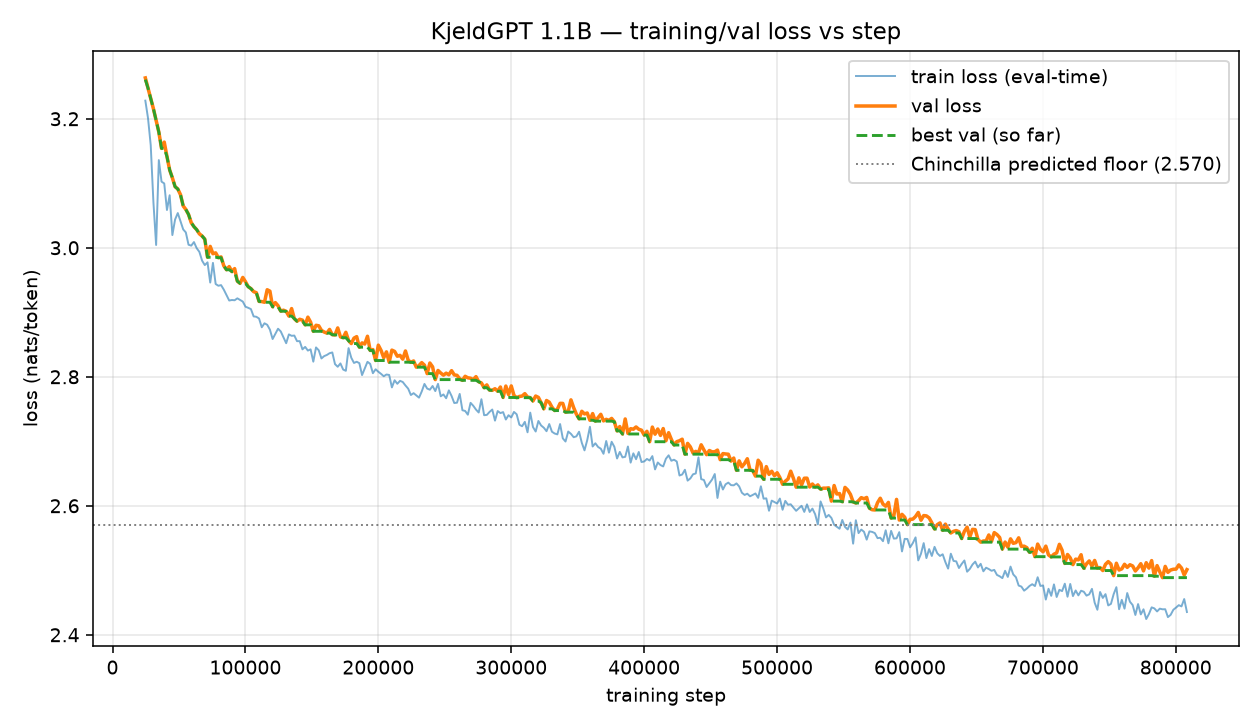
The train and val loss plotted above are cross-entropy loss when predicting the training and validation corpus. This means that when the model gets better the train and val loss get smaller.

One notices three things:

• Most of the improvements take place in the first part of the training. This is expected based on the power laws that govern GPT training.
  
  
• One also sees that my training actually achieved a lower validation loss than the Chinchilla-derived estimate. As the Chinchilla paper outlines general metrics for training GPT models, this is also not something fundamentally alarming.
  
  
• Finally, the improvements in train and val loss followed each other, with the model being consistently better at predicting the training corpus than the validation corpus. This is normal, and since the gap does not increase late in the training, there is no indication of overfitting.

I also plotted the val loss on a log-log graph against the compute used. This highlights the power law, as it produces a straight line in such a graph:

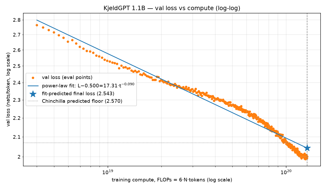
One notices that the training fit the power law quite well. What stands out is the apparent improved learning late in the training, where the training outperforms the power law fit.

What the Kaplan and Chinchilla papers outline is the optimal sizing for a given compute budget. This does not mean that the model, given more training than the initial budget allowed, will not further improve, but that this additional budget could have been used more effectively by training a larger model. But I did continue the training for an additional day, which confirmed the overall sizing of the model – the improvements after the 800,000th iteration were so small that training at that point had become ineffective.

The result

After 8 days of training I had a 1.1B parameter model capable of producing completions. The result is somewhat underwhelming when used to work with modern chat models:

As one can see the model is capable of producing completions that on the surface are somewhat coherent English, but is fundamentally a jumbled mess. The model has picked up English language syntax and there also appears to be glimpses of facts within the completions. But in general, the model — at this point — is pretty useless.

This is exactly the concept of pre-training, or base training, of a GPT. The model is now trained on a large corpus of English language texts, and has learned many of the statistical patterns of English and encoded some factual associations from its training corpus. But finetuning is needed to unlock the model’s capabilities. In the next post I will describe how this is done.